Christopher Monckton and Projecting Future Global Warming, Part 1

The outline for this post is as follows:

1. Introduction
2. Summary of the Objections
3. Elaboration on the Objections
4. References

This is part 1 of a two part series; part 2 will posted soon. If you want the "tl;dr" for this post, then I suggest reading sections 1 and 2. Alternatively, if you are familiar with Christopher Monckton's claims on climate sensitivity, then simply skip ahead to section 2.

Each numbered point in section 2 corresponds with a numbered portion of section 3. So there is no need to read this entire post; instead, you can see which numbered point you find interesting in section 2, and then for further details you can skip to the corresponding numbered portion in section 3.

This is the "main version" of this post, which means that this post lacks most of my references and citations. If you would like a more comprehensive version with all the references and citations, then please go to the "+References" version of this post.

References are cited as follows: "[#]", with "#" corresponding to the reference number given in the References section at the end of this post.

1.  Introduction

Earth's atmosphere contains multiple layers. The layer closest to the Earth's surface air is known as the troposphere. Above the troposphere is the stratosphere. Climate models and basic physical theory predict how carbon dioxide (CO2) will affect temperature trends in the troposphere and stratosphere. I addressed some of these predictions in my two part series on "John Christy and the Tropical Tropospheric Hot Spot" (part 1 and part 2), and in my post John Christy, Climate Models, and Long-term Tropospheric Warming".

Climate scientists attempt to estimate how much tropospheric and surface warming will result from a given increase in atmospheric CO2. This leads to estimates of climate sensitivity (CS), where CS is the increase in global average temperature for a doubling of atmospheric CO2 levels. Various processes serve as either positive feedback that increases CS or negative feedback that limits CS. Equilibrium climate sensitivity (ECS) is Earth's CS when Earth is in an equilibrium state where Earth releases as much energy as it takes in, and fast feedbacks (as opposed to slower acting feedbacks) have exerted their full effect. Transient climate sensitivity (TCS or TCR) is Earth's CS over a shorter period of time, before Earth reaches equilibrium. Different scientists give different definitions for CS and ECS, but the aforementioned definitions should suffice for this blogpost.

Scientists estimate CS in a number of ways, including:

• Paleoclimate records: This involves using proxies to estimate CO2 levels and temperature in the distant past. Scientists can then use these data to estimate CO2's effect on temperature.

• Historical / instrumental records: Similar to paleoclimate records, except scientists examine CO2 levels and temperature in the recent past, as opposed to the distant past.

• Climate models: Scientists generate climate models that are consistent with known physical laws, paleoclimate data, historical data, laboratory experiments performed on greenhouse gases such as CO2, and so on. These climate models range from very simple models generated in the 1800s, through more sophisticated models developed from the 1930s through the 1970s, to the complex climate models of today. Scientists compare these models to paleoclimate and historical data, to see which models best explain (or hindcast) the data. Scientists then use these validated models to project how much warming will result given increase in atmospheric CO2. This is consistent with standard scientific practice, since scientists in other fields justifiably use models to make projections about complex natural phenomena. For instance, oncologists can use biological models to project the likelihood that smokers will get lung cancer, despite the fact that oncologists do not know all of the biological processes involved in lung cancer. And astronomers generate astronomical models that fit with well-established physical laws and explain the motion of planets/satellites; astronomers then use those models to predict the motion of other planets/satellites, even though these models do not factor in the gravitational effect of every object in the universe. Similarly, climate scientists can use climate models to project how much warming will result from a given increase in CO2, even if climate scientists do not fully understand every process involved in global warming.

The following 2013 figure from the United Nations Intergovernmental panel on Climate Change (IPCC) shows some recent estimates of TCR and ECS based on the estimation methods I discussed above [1, figure 10.20 on page 925]:

Figure 1: Estimates of (a) TCR and (b) ECS from the scientific literature. The histogram height is proportional to the relative probability that CS is at the value shown on the horizontal axis. For example, the bottom panel on (b) includes Aldrin et al. 2012, where the maximum value for the histogram is around 1.7K, indicating that 1.7K is the most likely value for ECS of all possible ECS values examine in Aldrin et al. 2012. Horizontal bars show the probability range and the circles mark  the median estimate. The dashed lines in (a) show estimates from a previous IPCC report (AR4). The boxes on the right-hand side indicate limitations and strengths of each line of evidence. A blue box implies an overall line of evidence that is well understood, has small uncertainty, or many studies and overall high confidence. Pale yellow indicates medium confidence, and dark red implies low confidence [1, figure 10.20 of page 925].

I discuss some other recent CS estimates in section 3.1. Scientists have made progress with respect to estimating CS, though research continues on this subject. Many critics of mainstream climate science argue for low estimates of CS. These low estimates serve at least two purposes. First, they undermine public confidence in high estimates of CS, including the higher estimates offered by the IPCC. Second, the lower CS estimates (supposedly) suggest that anthropogenic global warming may not be very serious, since anthropogenic CO2 will cause less global warming than scientists initially thought. So these low CS estimates imply that anthropogenic global warming would be "lukewarm." Thus lukewarmers are critics who claim that less anthropogenic global warming will occur due to a low CS.

"Lord" Christopher Monckton is a prominent lukewarmer. Monckton uses a simple energy budget climate model to argue for a low ECS of 1.0K, in a paper Monckton co-authored with Willie Soon, David Legates, and William Briggs. Richardson et al. then wrote a rebuttal Monckton et al.'s paper. Monckton et al. subsequently responded to this rebuttal. In this part 1 post I will respond to some of Monckton et al.'s claims; in a subsequent post (part 2) I will respond to some of their other points.

In their two papers, Monckton et al. make a number of claims, including:

• The IPCC uses general-circulation climate models (GCMs) that over-estimate the real rate of global warming. I will call this the model-data discrepancy, in keeping with my post "John Christy, Climate Models, and Long-term Tropospheric Warming". Monckton et al. use this model-data discrepancy to argue that the IPCC's 1990 temperature prediction over-estimated the rate of global warming.

• Temperature data fit better with the predictions of Monckton et al.'s simple energy budget model, as opposed to the predictions made by the GCMs used by the IPCC. This supports a lower CS, since Monckton et al.'s model implies a net negative feedback that limits global warming and keeps CS low.

• The IPCC's offers an unjustified temperature projection showing ~12K of extreme global warming in response to very high greenhouse gas emissions. This biased projection depends on over-estimating global population.

• There has been a pause/hiatus in significant global warming for about two decades and this pause/hiatus was not predicted by GCMs.

• The IPCC accepts that its short-term predictions failed. This raises questions about the IPCC's longer-term predictions. 

• The urban heat-island effect (UHI) involves surface temperature stations recording warming that results from urbanization, as opposed to a changing climate. UHI biases temperature station records, causing climate scientists to mistake UHI-induced warming for warming induced by climatic factors.

So let's go over some of the issues with Monckton et al.'s arguments.

2. Summary of the Objections

Monckton et al.'s arguments fail so miserably that neither of Monckton et al.'s two papers should have passed competent peer review. For instance, Monckton et al. blatantly misrepresent sources, as I discuss more in part 2. To borrow Monckton et al.'s response to Richardson et al.'s rebuttal [2, page 1387]:

Here, Monckton et al. are more than somewhat disingenuous.

Below is a brief summary of some of the shortcomings of Monckton et. al's arguments:


1) Monckton et al. used a flawed approach based on an energy budget model. This approach under-estimates CS, as do a number other CS estimates based on energy budget models. Correcting this flawed approach results in a higher estimate of CS, which conflicts with Monckton et al.'s lower CS estimate.

2) Monckton et al. remain unclear about how they generated their IPCC temperature predictions. This is a problem because Monckton has a history of misrepresenting IPCC temperature projections. Monckton et al. partake in this history of misrepresentation by distorting the IPCC's temperature projections for a high emissions scenario. This distortion involves Monckton et al. under-estimating projected global population and over-stating the IPCC's projected warming trend.

3) Monckton et al. exaggerate the model-data discrepancy with respect to tropospheric temperature. They do this by excluding data that shows tropospheric warming, using outdated data sets, cherry-picking short time periods, offering misleading temperature graphs, and not paying adequate attention to other possible explanations of the model-data discrepancy. Addressing these errors results in less of a model-data discrepancy and a greater global warming trend. This warming trend argues against Monckton et al.'s lower CS. Furthermore, the IPCC's 1990 temperature model-based predictions were more accurate than Monckton et al. claim and more accurate than Monckton et al.'s hypothesized trend, as per sections 1 and 2.1 of "Myth: The IPCC's 1990 Report Over-estimated Greenhouse-gas-induced Global Warming".

4) Many climate models predicted a temporary slowdown in global warming and global warming has continued over the past two decade, contrary to the claims made by Monckton et al. This warming bears the hallmarks of CO2-induced global warming, in combination with ozone recovery. In order to generate a pause/hiatus in global warming, Monckton et al. engage in end-point bias, cherry-pick short-time periods, fail to adequately account for short-term variables that influence short-term trends, and fail to adequately address the effects of stochastic noise on small sample sizes. Monckton et al. also incorrectly claim that if the IPCC's shorter term temperature predictions fail, then this calls into question the IPCC's longer term projections. Monckton et al.'s reasoning makes little sense since various factors often bias short-term trends, without those factors also biasing long-term trends. Furthermore, as the IPCC itself notes, shorter term variability is often not representative of longer term trends. This shorter-term variability does not support Monckton et al.'s lower ECS estimate.

5) UHI does not strongly bias surface temperature trends in the way Monckton et al. claim, since data analysis (via homogenization) corrects for the effect of UHI, most of the surface warming trend remains even after UHI is factored out, surface warming trends in rural areas often match warming trends from urban areas, much of the most intense warming occurs in non-urbanized areas, scientists do not observe UHI's predicted effect on temperature on windy vs. non-windy days, and the ocean warming trend provides UHI-independent verification of the land warming trend.


Let's examine each of these objections in turn.

3. Elaboration on the Objections

3.1 Using an energy budget model to under-estimate CS

Energy budget models are one model-based approach for estimating CS. However, in comparison to other methods of estimating CS, energy budget models often generate lower estimates of CS due to a number of limitations, including under-estimating actual rates of historical warming and inaccurately representing the influence of aerosols on Earth's temperature. Correcting these errors results in higher estimates of climate sensitivity. So if you have ever heard a lukewarmer claim that they "showed CS was low using observational data," then the lukewarmer likely used an energy budget model plus observational data. It is therefore not surprising that Monckton et al. would opt for an approach based on an energy budget model, since this approach allows them to under-estimate CS.

3.2 Disregarding other plausible explanations of the model-observations discrepancy

Monckton et al. do not clearly explain how they generated their IPCC temperature projection for tropospheric temperature. This is especially important because Monckton has a history of misrepresenting IPCC's projections. Monckton's misrepresentations include treating projections as failed predictions. To explore this issue further, let's first distinguish between projections and predictions.

In climate science, a projection states what will likely happen, given a set of initial conditions. A prediction states what will actually happen. For example, take the following two simple projections made by James:

1. If Earl crosses the street at 17:00, then the red car will hit Earl.
2. If Earl does not cross the street at 17:00, then the red car will not hit Earl.

Suppose Earl does not cross the street at 17:00. One can plug this information into James' projections, and come up with the prediction that "The red car will not hit Earl." Now, suppose Monk said that:

"The red car did not hit Earl. So James was wrong when he predicted that the red car would hit Earl. James is thus an alarmist who tried to needlessly frighten Earl."

Monk's claim fails since James did not predict that Earl would be hit by the red car. Instead James projected that Earl would be hit by the car, if Earl crossed the street at 17:00. Since the "Earl crossed the street at 17:00" sufficient condition was not met, then James did not predict that Earl would be hit by the red car. Thus Monk conflated James' projection with James' prediction.

Monckton et al. commit this same misrepresentation. For example, Monckton et al. take climate projections made by the climate scientist James Hansen, and then imply that Hansen's projections do not match the observations. Of course, Monckton et al. fail to mention that Hansen's projections were based on sufficient conditions that were not met, and thus it would be unfair to treat these Hansen's projections as dis-confirmed predictions. Hansen's actual temperature prediction is more accurate than Monckton et al. imply.

Monckton misrepresents temperature projections in other ways, including:

• Treating the IPCC's ECS estimates as being equivalent to TCS estimates.

• Incorrectly treating average centennial temperature projections as being directly translatable into linear, decadal trend predictions. This makes no sense since shorter, decadal time periods are more prone to the effects of short-term factors and stochastic noise, and thus one not necessarily expect a decadal temperature trend to be a match the average centennial trend (for more on this see section 3.4, see sections 3.3 and 3.4 of John Christy, Climate Models, and Long-term Tropospheric Warming)

Given this history of misrepresentation, it should be no surprise that Monckton et al. misrepresent IPCC projections for the RCP8.5 (representative concentration pathway) scenario. RCP8.5 is a high emissions scenario, where humans continue to burn fossils in a "business-as-usual" manner. Monckton et al. claim that the IPCC RCP8.5 scenario projects 12K of warming by 2100, if humans burn all the recoverable fossil fuel reserves. Monckton et al. provide no evidence in support their claim. Furthermore, I cannot find any evidence that the RCP8.5 involves human burning all the recoverable fossil fuel reserves in a way that leads to 12 K of warming. Instead RCP8.5 depicts a "relatively conservative business as usual case with low income, high population and high energy demand due to only modest improvements in energy intensity," with a surface temperature increase of no more than 8K by 2100. So Monckton et al. likely generated the 12K projection by illegitimately extending the RCP8.5 projection outside of RCP8.5's sufficient conditions.

Monckton et al. also claim that RCP8.5 likely over-estimates the size of Earth's future population:

"Fifthly, application of the simple model raises the question why AR5 adopted the extreme RCP 8.5 scenario at all. On that scenario, atmospheric CO2 concentration is projected to reach 936 ppmv by 2100 on the basis of two implausible assumptions: first, that global population will be 12 billion by 2100, though the UN predicts that population will peak at little more than 10 billion by not later than 2070 and will fall steeply thereafter [...] [3, pages 133 and 134]."

This is false. The UN projects global temperature to be just below 11 billion by 2100, with a population of 12 billion being well within the range of plausible values. Furthermore, a 2100 global population of 12 billion is within the range of values presented in the scientific literature on emissions scenarios. These points are illustrated in figures 2A and 3 (top right panel) below:

Figure 2: (A) Top panel: UN 2012 world population projection (solid red line), with 80% prediction interval (dark shaded area), 95% prediction interval (light shaded area), and the traditional UN high and low variants from adding or subtracting half a child from the total fertility rate (dashed blue lines). The prediction interval is the range of values that future data will fall into, with a given probability. (B) Bottom panel: UN 2012 population projections by continent. In both panels, the vertical dashed line denotes 2012 [4].

Figure 3: Global development of population in RCP 8.5 (red lines) compared to the range of scenarios from the literature (grey areas: database of scenarios used in the previous IPCC AR4 report). Right hand vertical lines give the AR4 database range in 2100, including the 5th, 25th, 50th, 75th, and 95th percentile of the IPCC AR4 scenario distribution [5].

In summary: there is little reason to think that Monckton et al. accurately represented IPCC temperature projections and predictions, given Monckton's history of misrepresenting IPCC's projections and Monckton et al.'s misleading claims about the RCP8.5 scenario. So one has little reason for accepting Monckton et al.'s claim that observed warming rates fit better with Monckton et al.'s model energy budget model as opposed to the IPCC's model-based predictions. This undermines Monckton et al.'s model-based rationale for a low CS estimate.

3.3 Over-estimating discrepancies between data and model-based predictions

Monckton et al. over-estimate the model-data discrepancy when it comes to tropospheric temperature data. Many of these exaggerations stem from Monckton et al. adapting a flawed graph made by the climate scientist John Christy. Correcting these exaggerations reduces the model-data discrepancy and augments the observed tropospheric warming trend. These corrections also show that Monckton et al.'s energy budget model under-estimates the observed tropospheric warming trend, and thus Monckton et al.'s model-based approach likely under-estimates CS.

Monckton et al. exaggerate the model-data discrepancy in at least the following ways (for more on these exaggerations, see the cited sections from "John Christy, Climate Models, and Long-term Tropospheric Warming"):

• Monckton et al. use an outdated satellite-based temperature analysis from Remote Sensing Systems (RSS) that contains a cold bias acknowledged by the RSS team; RSS corrected this bias in a later analysis. Monckton et al. also do not use an improved RSS analysis that shows greater tropospheric warming and they do not include a similar satellite-based analysis from a research team at the National Oceanic and Atmospheric Administration Center for Satellite Applications and Research (NOAA/STAR). This NOAA analysis also shows greater tropospheric warming. Incorporating this data would likely reduce Monckton et al.'s model-data discrepancy (sections 3.1 and 3.2).

• Monckton et al. do not use three satellite data analyses (RSS, NOAA, UAH (University of Alabama in Huntsville)) that were corrected for stratospheric cooling. These data analyses show augmented tropospheric warming globally and in the tropics, reducing the model-data discrepancy presented by Monckton et al. (sections 3.1 and 3.2).

• Monckton et al. do not use a satellite data analysis for the tropics from a research team at the University of Washington (UW). This analysis shows increased tropical tropospheric warming, further reducing Monckton et al.'s model-data discrepancy (sections 3.1 and 3.2).

• Monckton et al.'s analysis does not include weather balloon (radiosonde) temperature records and temperatures re-analyses that show tropospheric warming. Including this data would likely reduce the model-data discrepancy.

• Monckton et al. do not mention the spurious cooling in the radiosonde temperature records that they use, even though this cold bias was commented on in a report co-authored by Christy. Correcting this cold bias would reduce the model-data discrepancy (section 3.1).

• Monckton et al. average data-sets together, obscuring the observational uncertainty in the data. This uncertainty results from, in part, differences between data-sets. Properly depicting this observational uncertainty would reduce the model-data discrepancy, and show that much of the discrepancy is due to observational uncertainty, as opposed to errors in the GCMs (sections 3.3 and 3.6). Monckton et al. further obscure observational uncertainty by mentioning the UAH data analysis, without illustrating how much Christy's UAH results differ from the results of other research groups. These differences likely result from errors in UAH's data analysis, consistent with UAH's history of errors in satellite data analysis. The UAH team likely under-estimated the rate of tropospheric warming. Correcting UAH's errors would likely reduce the model-data discrepancy (sections 3.1 and 3.2).

• Monckton et al. do not adequately represent the structural uncertainty in GCM-based warming projections, and thus commit the same mistake as Christy. As with observational uncertainty, displaying model uncertainty would reduce the model-data discrepancy and show that this model uncertainty explains much of the model-data discrepancy (section 3.6).

• Monckton et al. suggest that the model-data discrepancy is likely due to GCMs over-estimating the real warming trend, and they canvass some possible explanations for this over-estimation. However, Monckton et al. do not pay sufficient attention to other plausible alternative explanations for the discrepancy; observational uncertainty is one such alternative explanation, as is short-term variability. Scientific evidence supports these alternative explanations and these explanations do not imply a flaw in the GCMs (section 3.3). 

• Taking short-term variability into account shows the IPCC's 1990 temperature prediction was more accurate than Monckton et al. claim, as were other temperature mainstream temperature predictions. In fact, the IPCC's 1990 forecast was more accurate than Monckton et al.'s hypothesized trend, as per sections 1 and 2.1 of "Myth: The IPCC's 1990 Report Over-estimated Greenhouse-gas-induced Global Warming".

Other scientists avoided some of the aforementioned mistakes committed by Monckton et al. These scientists also avoided the Monckton et al. misrepresentations I discussed in section 3.2, such as inventing linear, decadal temperature predictions and then falsely attributing those predictions to the IPCC. Correcting Monckton et al.'s errors results in better graphs of the model-data discrepancy. Let's compare one of these graphs to a graph from Monckton et al.:

Figure 4: Mid- to upper tropical tropospheric warming trends predicted by climate models and observed in satellite data analyses. The pink line is the observed tropospheric warming trend, corrected for stratospheric cooling and shown as an average of the UAH, RSS, NOAA, and UW satellite data analyses. The black line shows the average warming trend from an ensemble of climate models, while the gray region shows the range of values taken by different realizations of each model [6].

Figure 5: Tropical mid-tropospheric temperature trends from 1979 to 2012, as predicted by climate models, with observations from radiosonde and satellites [2].

Figure 5 differs markedly from the corresponding figure 4, even though both figures purport to compare tropical mid-tropospheric temperature trends in observations vs. model predictions. Figure 5 exaggerates the model-data discrepancy in a way figure 4 does not. The remaining model-data discrepancy in figure 4 are likely due to a number of factors, including factors other than the models over-estimating CS (ex: factors such as observational uncertainty and model uncertainty).

The tropical upper tropospheric warming trends (in K per decade) for the four satellite data analyses in figure 4 are as follows:

• RSS  :  ~0.18
• NOAA  :  ~0.20
• UW  :  ~0.16
• UAH  :  ~0.10

So UAH is clearly the outlier, as I mentioned previously mentioned.

(The RSS, NOAA, and UW trends are fairly consistent with 5 out of 6 radiosonde trends for 1979-2014 and 2 out of 3 temperature re-analyses from 1979-2012 (in K per decade):

• Five radiosonde analyses each generally have upper tropospheric temperature trends of  :  >0.17
• Met Office Hadley Centre (HadAT2) radiosonde analysis  :  >0.11
• Modern Era Retrospective-Analysis for Research and Applications (MERRA) re-analysis  :  ~0.26
• European Centre for Medium-Range Weather Forecasts Interim re-analysis (ERA-I)  :  ~0.22
• National Centers for Environmental Prediction (NCEP-2) re-analysis  :  ~0.08

The NCEP-2 re-analysis has a history of under-estimating tropospheric warming, so the low NCEP-2 trend should be taken with a grain of salt. ERA-I likely under-estimates lower tropospheric warming. And even though the radiosonde analyses have a well-known cold bias, 5 of the 6 radiosonde trends are more consistent with the higher RSS/NOAA/UW satellite trend that the lower UAH trend.)

To compare these figures to Monckton et al.'s graph in figure 5, let's average the satellite temperature trends together (with or without the outlier UAH trend), and then multiply this average trend by 3.6 to convert the average trend into an average temperature increase from 1979 to 2015:

• Average temperature increase without UAH  :  ~0.65K
• Average temperature increase with UAH  :  ~0.58K

Both of these temperature increases are over twice as large as the ~0.25K increase (by 2015) shown by Monckton et al. in figure 5 above. So Monckton et al. under-estimate tropical tropospheric warming and thus exaggerate the model-data discrepancy. Fixing this exaggeration reduces the model-data discrepancy, and shows that Monckton et al.'s model-based approach likely under-estimates CS, in virtue of their model under-estimating the observed tropospheric warming trend.

3.4 Cherry-picking short time periods to generate a pause/hiatus in global warming

Monckton et al. select short time-frames for examining RSS data and claim that models failed to predict a period of almost two decades without significant global warming. In making these claims, Monckton et al. again repeat the same errors made by John Christy. I discuss some of these mistakes in sections 3.4 and 3.5 of "John Christy, Climate Models, and Long-term Tropospheric Warming". Here is a summary of some of the errors committed by Monckton et al.:

• Monckton et al.'s cherry-picking of short-term variability, does not change the long-term global warming trend and does not show that long-term global warming underwent a "pause/hiatus". One can justifiably investigate short-term variability and the factors influencing short-term trends, while accepting that there is an underlying, long-term global warming trend. So, for example, the same data that shows long-term global warming and global warming over the past 18 years, can also be used to investigate the short-term climate variability that temporally dampens the rate of global warming. This point remains compatible with skepticism about the existence of a recent, significant pause/hiatus in global warming. One would expect variability to temporally augment or mitigate a long-term global warming trend; therefore, it is not surprising that the rate of global warming temporarily decreased after the late 1990s. Such behavior occurred in past warming periods and climate model simulations, contrary to the false claims of Monckton et al. Scientists have commented on past periods of mitigated warming since at least the 1980s. No doubt future "skeptics" will follow Monckton et al.'s example by cherry-picking periods of mitigated warming and using these periods of argue for a "pause/hiatus" in global warming.

• Though some disagreement remains, models incorporating short-term natural variability (such as ENSO) and CO2-induced global warming have done better at modelling the current warming period, especially with respect to ocean warming. One would expect such a result if short-term variability temporarily augmented or mitigated a long-term, CO2-induced global warming trend. This is somewhat analogous to explaining average Canadian temperature from mid-winter to mid-summer by having short-term, multi-day or multi-week weather patterns layered on top of long-term, multi-month warming caused by changes in Earth's axial tilt relative to the Sun (I discuss this analogy further in section 3.4 of "John Christy, Climate Models, and Long-term Tropospheric Warming").

• Monckton et al. cherry-picked a warm start point (1997-1998) for their trend and made sure that the start point was biased by a short-term fluctuation. This short-term fluctuation is the El Niño phase of ENSO, an ocean cycle in which the oceans' surface and the troposphere temporarily warm. Scientists and non-scientists emphasize the dangers of choosing short-term trends that begin with a strong El Niño year like 1998, especially given the 1998 transition in satellite temperature monitoring equipment. The RSS team repeat this warning, as do Richardson et al., but to no avail; Monckton et al. cherry-pick anyway. To address the effect of ENSO, scientists also often examine temperature trends after correcting for short-term cyclical factors such as ENSO. Correcting for ENSO reveals the underlying long-term global warming trend, a trend that continues over the last two decades; tropospheric temperatures increased from 1997-1998 to 2015-2016, even though the 1997-1998 El Niño was about as strong as (or possibly stronger than) the 2015-2016 El Niño in terms of warming of the ocean surface (with the 2015-2016 El Niño having less ocean warming in some regions, and greater ocean warming in other regions, than did the 1997-1998 El Niño).

• There has been global warming over the past couple of decades, as observed in surface and ocean warming, tropospheric warming, and Earth's energy balance (the amount of energy the Earth takes up vs. the amount of energy the Earth releases). This warming runs contrary to Monckton et al.'s of no recent global warming. Recent warming bears the hallmarks of CO2-induced global warming, in combination with ozone stabilization. Namely: ozone depletion and increased CO2 caused stratospheric cooling up to the mid-1990s, as predicted by the scientific community during the 1960s, 1970s, and 1980s. Atmospheric warming caused by ENSO or the Sun would not produce most of the stratospheric cooling that has been observed. Ozone stabilization (in response to international treaties such as the Montreal Protocol) mitigated lower stratospheric cooling from the mid-1990s to the present, though recent stratospheric cooling remains in many data-sets, especially higher in the stratosphere. This is in agreement with scientific predictions made in the 1970s and 1980s. Increased CO2 levels also caused a shift in Earth's energy balance and greater absorption of energy (meaning increased radiative forcing) within specific infrared wavelengths that CO2 is known to absorb.

• Monckton et al. engage in end-point bias when they insinuate that a short-term temperature fluctuation paused a long-term warming trend. This is especially problematic since short-term factors can bias short-term trends, without those factors also biasing longer trends. Short-term trends can also be biased by chance / statistical noise, while larger sample sizes are not as prone to these effects. So shorter term variability is often not representative of longer term trends, as the IPCC itself notes. It is therefore unlikely that the IPCC would claim that the failure of short-term predictions implies a problem for long-term predictions. Yet Monckton et al. imply the opposite; Monckton et al. raise questions about the IPCC's longer-term predictions, because Monckton et al. claim (without any citation to the IPCC) that the IPCC accepts that its short-term predictions failed. Monckton et al.'s representation of the IPCC is difficult to reconcile with what the IPCC actually says:

"In addition to robust multidecadal warming, global mean surface temperature exhibits substantial decadal and interannual variability. Owing to natural variability, trends based on short records are very sensitive to the beginning and end dates and do not in general reflect long-term climate trends. As one example, the rate of warming over the past 15 years (1998–2012; 0.05 [–0.05 to +0.15] °C per decade), which begins with a strong El Niño, is smaller than the rate calculated since 1951 (1951–2012; 0.12 [0.08 to 0.14] °C per decade) [7, page 194]."

To make these points even clearer, let's examine RSS' mid-tropospheric temperature analysis and the HadCRUT surface temperature analysis [6; 8 - 10], since Monckton et al. rely on both of RSS and HadCRUT:

Figure 6: Trend in global, monthly, mean surface temperature from 1979 to 2016 relative to baseline of 1981 - 2010, as shown in multiple temperature analyses. The solid green trend-line is represents the trend for 1998 - 2012, while the dotted black trend-line represents the trend for the full period from 1979 - 2016 [13].

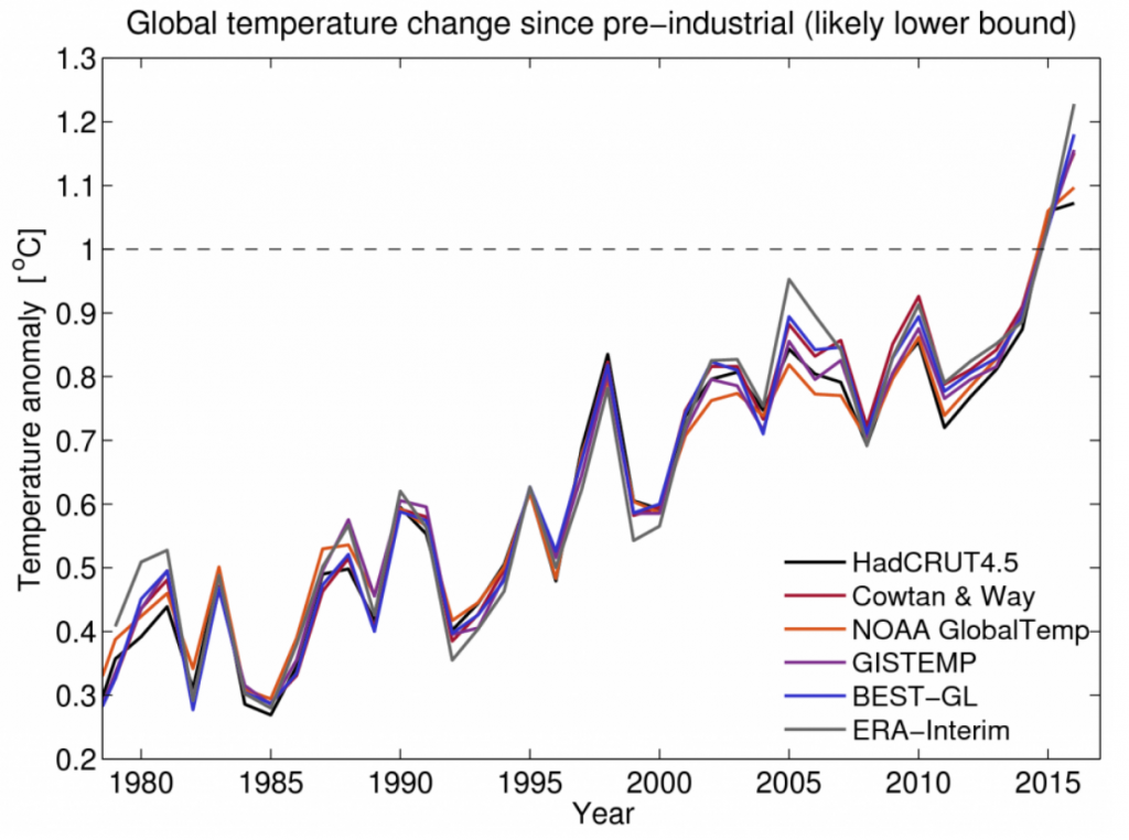Figure 7: Global, annual, mean surface temperature relative to baseline of 1981-2010 (1720 - 1800), or relative to mean temperature from 1986 - 2005 in the case of ERA-Interim [8], as shown in multiple temperature analyses. Pre-2016 data came from a previous scientific publication [8], with later data added in a subsequent work [9].

Figure 8: RSS near-global mid- to upper tropospheric temperature, with trend-lines for different 18 year periods [6].

Figure 9: Version 3.3 and version 4.0 of the RSS near-global lower tropospheric temperature analysis, along with version 5.6 and version 6.0 of the UAH near-global lower tropospheric temperature trends. RSS version 4.0 is an update of RSS version 3.3, while UAH version 6.0 is an update of UAH version 5.6. The lower lines (black, gray, red, and pink) indicate temperature relative to a baseline of 1979 - 1981. The upper lines (green and purple) display the difference between the relative temperature values. Quantified trends are from 1979 - 2016.

Figure 6 shows that the short-term temperature trend that begins with a strong El Niño (solid green line in figure 6) under-estimates the long-term warming trend (dotted black line in figure 6), in accordance with the IPCC's aforementioned assessment. Figure 8 also shows how one's start point and end-point greatly impact the magnitude of the short-term trend. For example, one can follow Monckton et al.'s example and have a strong El Niño year near one's chosen start point, while not having an El Niño near one's end-point. Such blatant cherry-picking allows Monckton et al. to generate and exploit a non-representative, short-term trend; this is analogous to choosing the short-term green trend in figure 6, over the long-term black trend in figure 6.

Figures 6 to 9 also show that 2016 was warmer, on average, than 1998. One might object that figure 4 from section 3.3 shows that 2016 is not warmer than 1997-1998. However, this objection is incorrect. Figure 4 depicts upper tropospheric warming in the tropics. When one examines the near-global upper tropospheric trend, then it becomes clear that 2016 was warmer, on average, than 1998 [11]:

Figure 10: Near-global mid- to upper tropospheric temperature averaged for the UAH, NOAA, and RSS analyses [11]. 

So figures 6 to 10 show a warming trend from 1998 to 2016. Once again, this warming trend is not wholly attributable to ENSO, since the El Niño of 2015-2016 was about as strong as (or weaker than) the El Niño of 1997-1998 in terms of warming of the ocean surface (with the 2015-2016 El Niño having less ocean warming in some regions, and greater ocean warming in other regions, than did the 1997-1998 El Niño). So if one wanted to investigate the underlying global warming trend, then comparing 1998 to any subsequent year other than an equally strong El Niño year (such as 2016) would be misleading, since ENSO would skew the start point for that short-term trend. This confirms that the global warming trend remains even after correcting for ENSO, as shown in other sources.

The underlying global warming trend is largely caused by CO2. To see why, first note that since the 1800s, atmospheric CO2 levels increased in a roughly exponential manner. Given the logarithmic relationship between increase CO2 and increased temperature, this near-exponential increase in CO2 caused a near-linear CO2-induced warming trend, though the linearity breaks down in extreme cases. Short-term variability (from factors such as ENSO) and chance / statistical noise temporarily augmented or mitigated this linear warming trend , as depicted in figures 6, 8, and 9. Figure 10b depicts the linear warming trend more clearly, with much of the short-term variability removed [12]:

Figure 11: (a) Global surface temperature trend from 1856 - 2010 after correcting for TSI (total solar irradiance, a measure of the solar radiation reaching Earth), ENSO, and volcanic aerosols. The upper-left, boxed inset depicts a measurement of the Atlantic multi-decadal oscillation (AMO), a cycle that affects ocean temperatures. (b) Global surface temperature trend after correcting for the AMO, TSI, ENSO, and volcanic aerosols [12]. 
It unclear whether the AMO is an independent cause of ocean warming vs. the AMO being a type of ocean warming caused by other factors. There is also some dispute over whether the AMO impacts temperature as strongly as is shown panel (b). For instance, aerosols, instead of the AMO, may have partially offset CO2-induced warming during the 1940s to 1970s. Some sources attribute much of the recent warming to the AMO, while other sources argue that the AMO does not account for much of the recent warming. In either case, greenhouse gases such as CO2 substantially contributed to recent global warming. And since the post-1964 multi-decadal global warming trend extends over more than 50 years, the 30-year increasing portion of the roughly 60-year AMO cycle may not account for such a long warming trend.

So it would be misleading to cherry-pick a short period of mitigated global warming, in order to argue accurate estimates of the long-term CO2-induced warming trend. But this fact did not stop Monckton et al. from cherry-picking a two-decade long period of reduced global warming, in order to argue against GCM-based projections of CO2-induced warming. Monckton et al.'s cherry-picking does not change the fact that global warming has occurred over the past two decades, nor does it change the fact that short-term temperature fluctuations should not undermine confidence in GCM-based temperature predictions. Monckton et al.'s cherry-picking also fails to support their CS estimate. Instead, incorporating the recent warming period still supports higher CS estimates, even if one does not take into account all of the other factors that cause CS to be under-estimated (factors I discussed in section 3.1).

3.5 Misattributing global warming to increased heat from urban development

Monckton et al. suggest that urbanization warmed much of the Earth surface. This is known as the urban heat-island effect (UHI). According to Monckton et al., some scientists then attributed this non-climatic warming to anthropogenic greenhouse gases, resulting in over-estimation of the warming caused by anthropogenic greenhouse gases. Monckton et al. support their claim by citing Michaels and McKitrick's research correlating economic growth with warming. However, other scientists critiqued Michaels and McKitrick's work, suggesting that their correlations were spurious. So Michaels and McKitrick's research may not provide a solid basis for claiming that UHI strongly biased measurements of CO2-induced global warming. When scientists examine other lines of evidence, it becomes clear that UHI does not strongly bias the surface temperature record. This can be shown through a number of means, including:

• Scientists use homogenization to correct for UHI. Homogenization is a process for correcting inhomogeneities, which are factors that artificially skew temperature records. I discuss and defend homogenization further in section 3.1 of "John Christy, Climate Models, and Long-term Tropospheric Warming". When one corrects for UHI, there is still statistically significant surface warming and most of the observed surface warming remains.

• The global warming trend is often not significantly higher in urban areas vs. rural areas. When there is a significant difference, homogenization can correct for this urbanization-induced difference. And much of the intense global warming occurs in non-urban, desertified areas in response to CO2-induced warming, or in non-urban areas in the Arctic. Therefore UHI would not strongly bias these intense warming trends.

• Wind mitigates the effect of UHI. So if UHI was responsible for much of the long-term warming, then there should be a large discrepancy in the temperature record for windy areas vs. non-windy areas. However, this predicted difference is not observed. Thus UHI is not responsible for much of the long-term warming trend.

• Scientists can validate and constrain land surface temperature records using other data sources. For example, satellite-based skin temperature analyses confirm the surface warming trend, as do proxy-based estimates, and other indirect estimates that do not use instrumental surface temperature data. Moreover, UHI should not significantly bias ocean temperature records since oceans are not urban. And ocean warming should be less than land warming, since oceans have a greater heat capacity than land. Ocean surface warming thus sets a UHI-independent lower limit for land surface warming. Scientists can also use climate models to predict the ratio of ocean surface warming to land surface warming. This ratio provides an UHI-independent upper limit for land surface warming. Land surface warming should significantly exceed this limit, if UHI substantially biased the land surface warming trend. Yet land surface warming is within this upper limit. This provides further confirmation that UHI has not substantially biased the global surface warming trend.

• The lukewarmer Anthony Watts argued that artificial heat from urban sources biased the temperature record of poorly run American temperature stations. So scientists at BEST (the Berkeley Earth Surface Temperature group) examined the warming trends in rural temperature stations approved of Watts vs. temperature stations Watts objected to. If UHI was responsible for much of the recent surface warming, then the warming trend in the rural stations should be significantly lower than the warming trend in the other stations. Yet the scientists observed no statistically significant difference between the two warming trends. This evidence, along with additional lines of evidence, changed the mind of Richard Muller, one of the BEST scientists performing this UHI research. In contrast, BEST's evidence did not change Watts' mind, despite the Watts' claim that he would accept BEST's results even if BEST's evidence showed Watts was wrong. And Watts' mind still did not change, even when research (including research Watts himself co-authored) showed a similar warming trend for average temperature at stations Watts approved of vs. stations Watts objected to (a pattern similar to that observed in other regions of the world). This exemplifies Watts' habit of evading, and not changing his mind in response to, evidence that shows he is wrong (for further examples of Watts' habit, see section 3.2 of "John Christy, Climate Models, and Long-term Tropospheric Warming", along with section 3.1 of part 1 and section 3.4 of part 2 of my series on "John Christy and the Tropical Tropospheric Hot Spot"). Watts unwillingness to change his mind is a classic sign of a denialism, in contrast to scientific skeptics who change their mind in response to evidence.

• Take one of the worst cases of UHI: China. UHI may account for up to around a third of the surface warming trend in China, according to research cited by Watts. A number of scientists have shown that this number likely over-estimates UHI's contribution to China's surface warming record. But, for the sake of argument, suppose one accepts that UHI causes roughly a third of China's surface warming trend. And then suppose one removes this estimated UHI-induced warming from the Chinese warming trend. Then China's warming trend closely matches the average global warming trend. So China, one of the worst cases of UHI, gives one little reason for thinking that UHI substantially skews the average, homogenized, global warming trend. 

Thus Monckton et al. were wrong when they suggested that UHI caused much of the recent surface warming and that UHI substantially contributed to over-estimation of the magnitude of anthropogenic global warming. Monckton et al. will need to find some other way of reducing the surface warming trend in way that fits with their low CS estimate.

4. References

1. "Climate change 2013: Working Group I: The physical science basis; Chapter 10; Detection and attribution of climate change: from global to regional"
2. "Keeping it simple: the value of an irreducibly simple climate model"
3. "Why models run hot: results from an irreducibly simple climate model"
4. "World population stabilization unlikely this century"
5. "RCP 8.5—A scenario of comparatively high greenhouse gas emissions"
6. "Comparing tropospheric warming in climate models and satellite data"
7. "Climate change 2013: The physical science basis; Chapter 2: Observations: Atmosphere and Surface"
8. "Estimating changes in global temperature since the pre-industrial period"
9. "Guest post: The challenge of defining the ‘pre-industrial’ era"
10. http://images.remss.com/msu/msu_time_series.html (accessed June 5, 2017)
11. "Tropospheric warming over the past two decades"
12. "Deducing multidecadal anthropogenic global warming trends using multiple regression analysis"
13. "A reassessment of temperature variations and trends from global reanalyses and monthly surface climatological datasets"